|
|
Overview
 IPM is a portable profiling infrastructure for parallel codes. It
provides a low-overhead performance profile of the performance aspects
and resource utilization in a parallel program. Communication,
computation, and IO are the primary focus. While the design scope
targets production computing in HPC centers, IPM has found use in
application development, performance debugging and parallel computing
education. The level of detail is selectable at runtime and presented
through a variety of text and web reports.
IPM has extremely low overhead, is scalable and easy to use requiring
no source code modification. It runs on Cray XT.s, IBM SP's, most
Linux clusters using MPICH/OPENMPI, SGI Altix and the Earth
Simulator. IPM is available under an Open Source software license
(LGPL). It is currently installed on several Teragrid, Department of Energy, and other
supercomputing resources.
IPM brings together several types of information important to
developers and users of parallel HPC codes. The information is
gathered in a way the tries to minimize the impact on the running
code, maintaining a small fixed memory footprint and using minimal
amounts of CPU. When the profile is generated the data from individual
tasks is aggregated in a scalable way.
For downloads, news, and other information, visit our Project Page. The
monitors that IPM currently integrates are:
IPM is a portable profiling infrastructure for parallel codes. It
provides a low-overhead performance profile of the performance aspects
and resource utilization in a parallel program. Communication,
computation, and IO are the primary focus. While the design scope
targets production computing in HPC centers, IPM has found use in
application development, performance debugging and parallel computing
education. The level of detail is selectable at runtime and presented
through a variety of text and web reports.
IPM has extremely low overhead, is scalable and easy to use requiring
no source code modification. It runs on Cray XT.s, IBM SP's, most
Linux clusters using MPICH/OPENMPI, SGI Altix and the Earth
Simulator. IPM is available under an Open Source software license
(LGPL). It is currently installed on several Teragrid, Department of Energy, and other
supercomputing resources.
IPM brings together several types of information important to
developers and users of parallel HPC codes. The information is
gathered in a way the tries to minimize the impact on the running
code, maintaining a small fixed memory footprint and using minimal
amounts of CPU. When the profile is generated the data from individual
tasks is aggregated in a scalable way.
For downloads, news, and other information, visit our Project Page. The
monitors that IPM currently integrates are:
- MPI: communication topology and statistics for each MPI call and buffer size.
- HPM: PAPI (many) or PMAPI (AIX) performance events.
- Memory: wallclock, user and system timings.
- Switch: Communication volume and packet loss.
- File I/O: Data written and read to disk
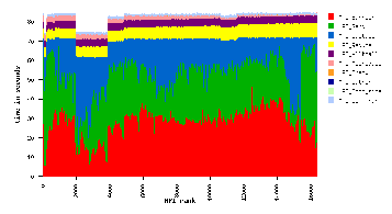
Aside from overall performance, reports are available for load
balance, task topology, bottleneck detection, and message size
distributions. Examples are sometimes better than explanation.
The 'integrated' in IPM is multi-faceted. It refers to binding the
above information together through a common interface and also the
integration of the records from all the parallel tasks into a single
report. At a high level we seek to integrate together the information
useful to all stakeholders in HPC into a common interface that allows
for common understanding. This includes application developers,
science teams using applications, HPC managers, and system architects.
IPM is a collaborative project between NERSC/LBL and SDSC. People
involved in the project include David Skinner, Nicholas Wright, Karl
Fuerlinger and Prof. Kathy Yelick at NERSC/LBNL and Allan Snavely at
SDSC.
|

 IPM is a portable profiling infrastructure for parallel codes. It
provides a low-overhead performance profile of the performance aspects
and resource utilization in a parallel program. Communication,
computation, and IO are the primary focus. While the design scope
targets production computing in HPC centers, IPM has found use in
application development, performance debugging and parallel computing
education. The level of detail is selectable at runtime and presented
through a variety of text and web reports.
IPM has extremely low overhead, is scalable and easy to use requiring
no source code modification. It runs on Cray XT.s, IBM SP's, most
Linux clusters using MPICH/OPENMPI, SGI Altix and the Earth
Simulator. IPM is available under an Open Source software license
(LGPL). It is currently installed on several Teragrid, Department of Energy, and other
supercomputing resources.
IPM brings together several types of information important to
developers and users of parallel HPC codes. The information is
gathered in a way the tries to minimize the impact on the running
code, maintaining a small fixed memory footprint and using minimal
amounts of CPU. When the profile is generated the data from individual
tasks is aggregated in a scalable way.
For downloads, news, and other information, visit our Project Page. The
monitors that IPM currently integrates are:
IPM is a portable profiling infrastructure for parallel codes. It
provides a low-overhead performance profile of the performance aspects
and resource utilization in a parallel program. Communication,
computation, and IO are the primary focus. While the design scope
targets production computing in HPC centers, IPM has found use in
application development, performance debugging and parallel computing
education. The level of detail is selectable at runtime and presented
through a variety of text and web reports.
IPM has extremely low overhead, is scalable and easy to use requiring
no source code modification. It runs on Cray XT.s, IBM SP's, most
Linux clusters using MPICH/OPENMPI, SGI Altix and the Earth
Simulator. IPM is available under an Open Source software license
(LGPL). It is currently installed on several Teragrid, Department of Energy, and other
supercomputing resources.
IPM brings together several types of information important to
developers and users of parallel HPC codes. The information is
gathered in a way the tries to minimize the impact on the running
code, maintaining a small fixed memory footprint and using minimal
amounts of CPU. When the profile is generated the data from individual
tasks is aggregated in a scalable way.
For downloads, news, and other information, visit our Project Page. The
monitors that IPM currently integrates are: